In the age of Big data and even Bigger models that readily consume data like a V-8 engine in a Dodge Charger guzzles through gas, it is even more critical to understand where these large Behemoths of models fail. Research on Adversarial Attacks is one of the few areas of Machine Learning which is not only mathematically interesting but has direct impact on real world systems. However, much of the theoretical interest in Adversarial Attacks has been largely focused on “Whitebox” settings where the adversary has complete access to the target model. Not only is this not realistic as in the real world models are often hidden beyond a security layer it also neglects many key aspects of the threat model that could promote new types of adversarial attacks.

In this Blogpost I’ll focus on a new kind of threat model that appears in a new NeurIPS 2020 Paper titled “Adversarial Example Games” which is joint work with a few amazing co-authors Gauthier Gidel, Hugo Berard, and other awesome collaborators, Andre Cianflone, Pascal Vincent, Simon Lacoste-Julien, William L. Hamilton. Motivated by real world use cases the paper focuses on a new type of adversary: NoBox Adversary which as the name suggests hints at a new attack strategy that works in more stringent threat models when compared to Whitebox or even conventional Query-based Blackbox threat models. To tease the rest of the blogpost, we will find that even when the attacker has no direct access to a target model —that means no queries— and might not even know the model architecture we can still construct adversarial attacks. In fact we can make an even stronger claim, we will be able to attack “all models” in a known function class simultaneously.

What are adversarial attacks?

The Adversarial Attack problem is deliciously simple to state, but for within the simplicity lies all the complexity which has resulted in thousands of papers. Let’s review the fundamentals of this problem here while an even more detailed blogpost can be found from the NeurIPS 2018 Tutorial on Adversarial Robustness. Suppose we are given a classifier \(f : \mathcal{X}\rightarrow \mathcal{Y}\), an input datapoint \(x \in \mathcal{X}\), and a class label \(y \in \mathcal{Y}\), where \(f(x) = y\). The goal of an adversarial attack is to produce an adversarial example \(x' \in \mathcal{X}\), such that \(f(x') \neq y\),

A classical way to frame this problem is through the lens of constrained optimization 1. That is, given a loss function \(\ell\), used to evaluate \(f\), a distance \(d\), an adversarial attack is said to be optimal if,

In practice, attack strategies that aim to solve this problem optimize for adversarial examples \(x'\) directly using the gradient of \(f\) and then evaluate the attack success rate (i.e., how often these \(x'\) successfully fool \(f\)).

The NoBox Threat Model

Threat models specify the formal assumptions of an attack (e.g., the information the attacker is assumed to have access to), which is a core aspect of adversarial attacks. In the NeurIPS 2020 Adversarial Example Games paper, we introduce the challenging setting of non-interactive blackBox (NoBox) attacks, intending to generate successful attacks against an unknown target crucially without query access. Let’s repeat what this means, we want to attack unknown target models, that means we won’t have access to its parameters and cannot take gradients to easily craft attacks like the WhiteBox setting. This is also harder than most BlackBox settings because the attacker only has one chance to attack the target model and they cannot adaptively craft their attack strategy based on the output of the target model. Given these intuitions, let’s formally state the NoBox threat model:

• The target model \(f_t\). The adversarial goal is to attack some target model \(f_t : \mathcal{X} \rightarrow \mathcal{Y}\), which belongs to an hypothesis class \(\mathcal{F}\). Critically, the adversary has no access to \(f_t\) at any time.
• The target examples \(\mathcal{D}\). The dataset \(\mathcal{D}\) contains the examples \((x,y)\) that attacker seeks to corrupt.
• An hypothesis class \(\mathcal{F}\). We assume that the attacker has access to a hypothesis class \(\mathcal{F}\) to which the target model \(f_t\) belongs.
• A reference dataset \(\mathcal{D_{ref}}\). The reference dataset, which is similar to the training data of the target model (e.g., sampled from the same distribution) is used to reduce the size of the hypothesis class.
• A representative classifier \(f_c\). Finally, we assume that the attacker has the ability to optimize a representative classifier \(f_c\) from the hypothesis class \(\mathcal{F}\).

In practice, the hypothesis class may include more information that some candidate architectures for \(f_t\). One can incorporate in \(\mathcal{F}\) as much prior knowledge one has on \(f_t\) e.g., the architecture, dataset, training method, or regularization.

Adversarial Example Games

The NoBox threat model presents a challenging new setting for adversarial attacks. How can one attack an unknown target model if we are unable to query it? At first such a proposition appears daunting but the devil is in the details. The NoBox threat model affords two key pieces of knowledge to the attacker: 1) A hypothesis class from which the target model is known to belong too 2) A representative classifier from this hypothesis class which is easily available to the adversary. At a high level one could hope to craft an attack on the target model by first crafting it on the representative classifier expecting it will transfer well to the target model. Initially there is no reason to suspect such a strategy should work at all, but empirically many have found such attack strategies termed “BlackBox transfer” attacks 2, 3, 4.

An intuition that one may have is that if we don’t know the specific target model we can then optimize for an attack that is “universal”, in that it cripples as many possible target models over the hypothesis class. Stated another way, we can think of crafting adversarial attacks against \(f \in \mathcal{F}\) as a two player game where the adversary proposes an attack and the opponent chooses a function from the hypothsis class which nullifies the attack —i.e. succesfully classifies the input. To formalize this a bit more we can view the attack generation task as a form of adversarial game. The players are the generator network \(g\)—which learns a conditional distribution over adversarial examples—and the representative classifier \(f_c\). The goal of the generator network is to learn a conditional distribution of adversarial examples, which can fool the representative classifier \(f_c\). In turn the representative classifier is optimized to detect the true label \(y\) from the adversarial examples generated by \(g\).

Overall, the generator \(g\) and the representative classifier \(f_c\) play the following, two-player zero-sum game:

The main insight from such a minimax formulation is that both the attack generator and representative classifier are jointly optimized and this process ensures generator’s adversarial distribution at the equilibrium theoretically effective against any classifier from the hypothesis class \(\mathcal{F}\). Another key insight is that if a Nash Equilibrium for this game exists then the order of min and max can be switched. This implies that The classifier network \(f_c\) is simultaneously optimized to perform robust classification over the resulting distribution \(p_{g}\) and converges to the best in class robust model. In the main paper we prove that under certain conditions such an equilibrium does in fact exist and later through experiments we empirically validate that attacks using this formulation can succefully attacks some of the strongest known defences.

Objective of the Generator

The goal of the generator can be seen as generating the adversarial distribution \(p_{g}\) with the highest expected conditional entropy \(\mathbb{E}_x[ \sum_y p_{g}(y|x) \log p_{g}(y|x)]\), where \(p_{g}\) is defined as

When trying to attack a specific hypothesis class \(\mathcal{F}\) (e.g., a particular CNN architecture), the generator aims at maximizing a notion of restricted entropy defined implicitly through the class \(\mathcal{F}\). Thus, the optimal generator is primarily determined by the statistics of the target dataset \(\mathcal{D}\) itself, rather any specifics of a target model. In a way the attack constructed is an attack on the data distribution itself!

Regularizing The Game

In practice, we can assume that \(f_t\) does well on classification on a non-adversarial dataset (what would be the point to attack a classifier that already performs poorly at the classification task?). Thus any representative classifier that the adversary samples should correspondingly be biased towards not only robust classification on the adversarial samples but also on regular vanilla classification. We can incorporate this notion and simultaneously reduce the size of the hypothesis class \(\mathcal{F}\) by adding a regularizer to overall AEG objective:

Note that \(\lambda=0\) recovers the original AEG formulation.

A Word on Theory

In the AEG paper we prove two main results. The first concerns the conditions for the existance of a Nash Equilibrium of the game and uses standard techniques in game theory (Fan’s theorem). More concretely, we prove the following minimax result:

Although a blog post is ill-suited to reproduce the main arguments it’s still constructive to mention the implications of such a result: At equilibrium we arrive at a best in class robust model and a corresponding attack generator that dominates all other models from this class. To craft attacks we simply take this trained generator and feed it inputs, \(x \sim \mathcal{D}\), leading to adversarial examples that simultaneously work against all models in the hypothesis class. If the generator is parametrized —i.e. like a Neural Net, then the inference cost is extremely cheap at test time and we can generate adversarial attacks on the fly circumventing cumbersome optimization on new unseen samples.

A Toy Example

Let’s take a simple logistic regression based classifier trained on the two moons dataset from sci-kit learn as an example. For features we will take linear, polynomials of degree 3 and 5 respectively. Note that we have \(\text{Linear} \subset \text{Poly3} \subset \text{Poly5}\). For simplicity, assume that it is possible to compute both the maximization and minimization. The figure below illustrates the effect of attacking each type of logistic regression classifier.

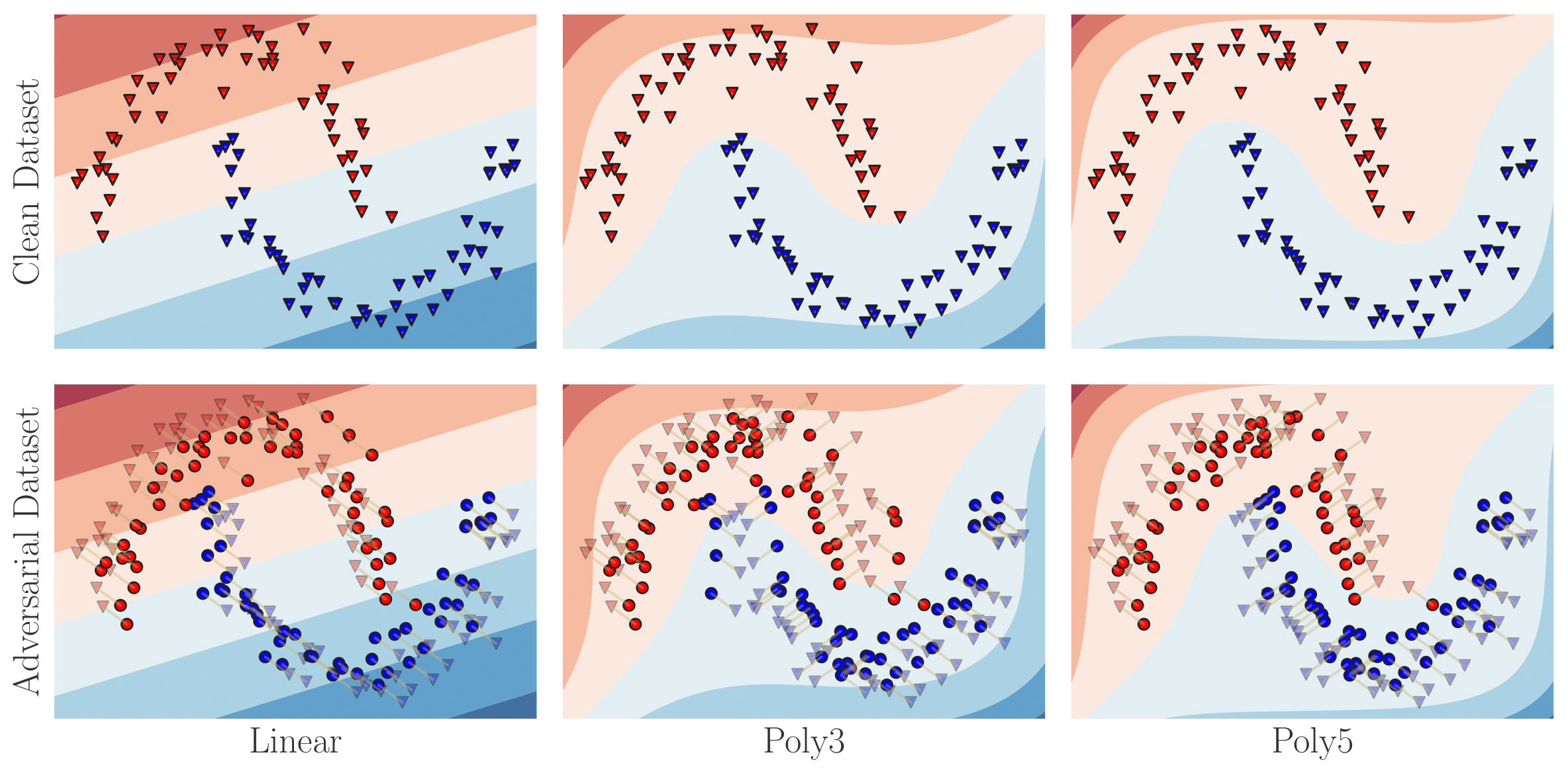For the adversarial dataset, each corresponding clean example is represented with a red/blue triangle and is connected to its respective adversarial example red/blue dot

The key observation from these figures is that the way of attacking a dataset depends on the class considered. For instance, when considering linear classifiers, the attack is a uniform translation on all the data-points of the same class. While when considering polynomial features, the optimal adversarial dataset pushes the the corners of the two moons closer together.

Adversarial attacks as “Entropy”-Maximization

As hinted at earlier in the blog post adversarial attacks in the NoBox threat model can be seen as an attack on the data distribution itself. One way to make this more concrete is to think about how stronger attacks increases the “entropy” over \(\mathcal{F}\). For a given distribution \((x,y) \sim p_{g}\) we can define the \(\mathcal{F}\)-entropy of \(p_g\) as

Here \(\ell\) is the cross entropy loss. Also, note \(\mathcal{F}\)-entropy is different from the usual definition of Entropy found in probability textbooks but it’s still a useful analogy. One of the main properties of \(\mathcal{F}\)-entropy —that we later prove in the paper— is the fact that \(\mathcal{F}\)-entropy is a decreasing function of \(\mathcal{F}\), i.e., for any \(\mathcal{F}_1 \subset \mathcal{F}_2\). As an example, we can plot the respective \(\mathcal{F}\)-entropies of the logistic regression classifiers considered above throughout the course of training.

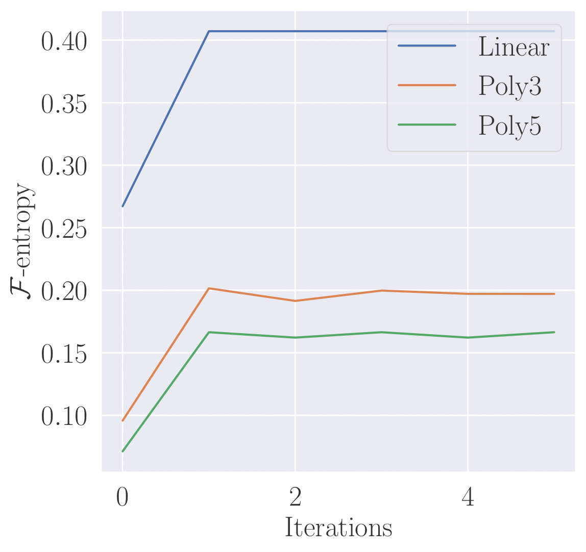
Unsurprisingly, AEG optimization increases the \(\mathcal{F}\)-entropy and also \(\mathcal{F}\)-entropy takes on a smaller value for larger classes of classifiers.

Attacking in the Wild

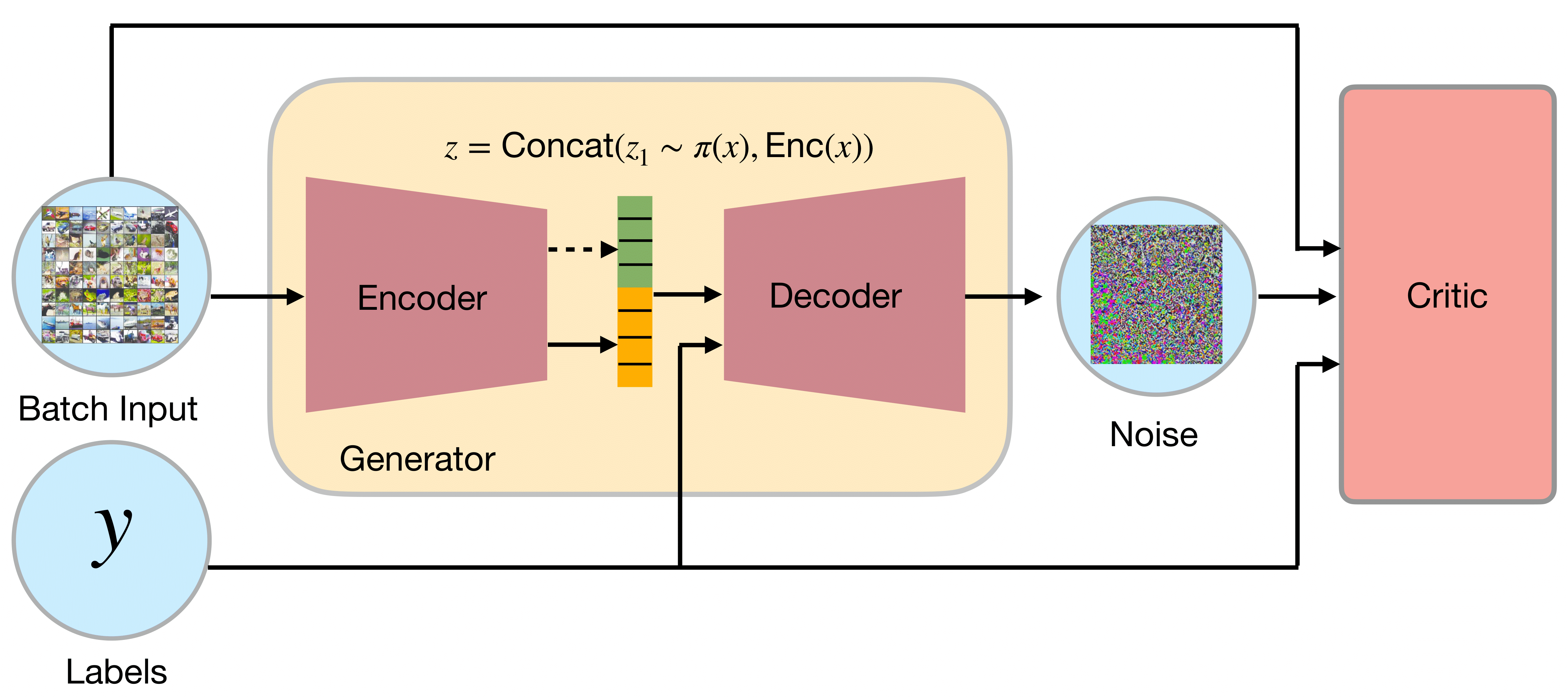
AEG Architecture

The high-level architecture of the AEG framework is illustrated below. The generator takes the input \(x\) and encode it into \(\psi(x)\), then the generator uses this encoding to compute a probability vector \(p(\psi(x))\) in the probability simplex of size \(K\), the number of classes. Using this probability vector, the network then samples a categorical variable \(z\) according to a multinomial distribution of parameter \(p(\psi(x))\). Intuitively, this category may correspond to a target for the attack. The gradient is backprogated across this categorical variable using the gumble-softmax trick. Finally, the decoder takes as input \(\psi(x)\), \(z\) and the label \(y\) to output an adversarial perturbation \(\delta\) such that \(\|\delta\|\leq \epsilon\).

NoBox Attacks between different architectures

The main paper investigates many experimental settings but for the purposes of this blogpost let us focus on one demonstrative setting: attacking target classifiers with different architectures than the representative classifier used to train the generator.

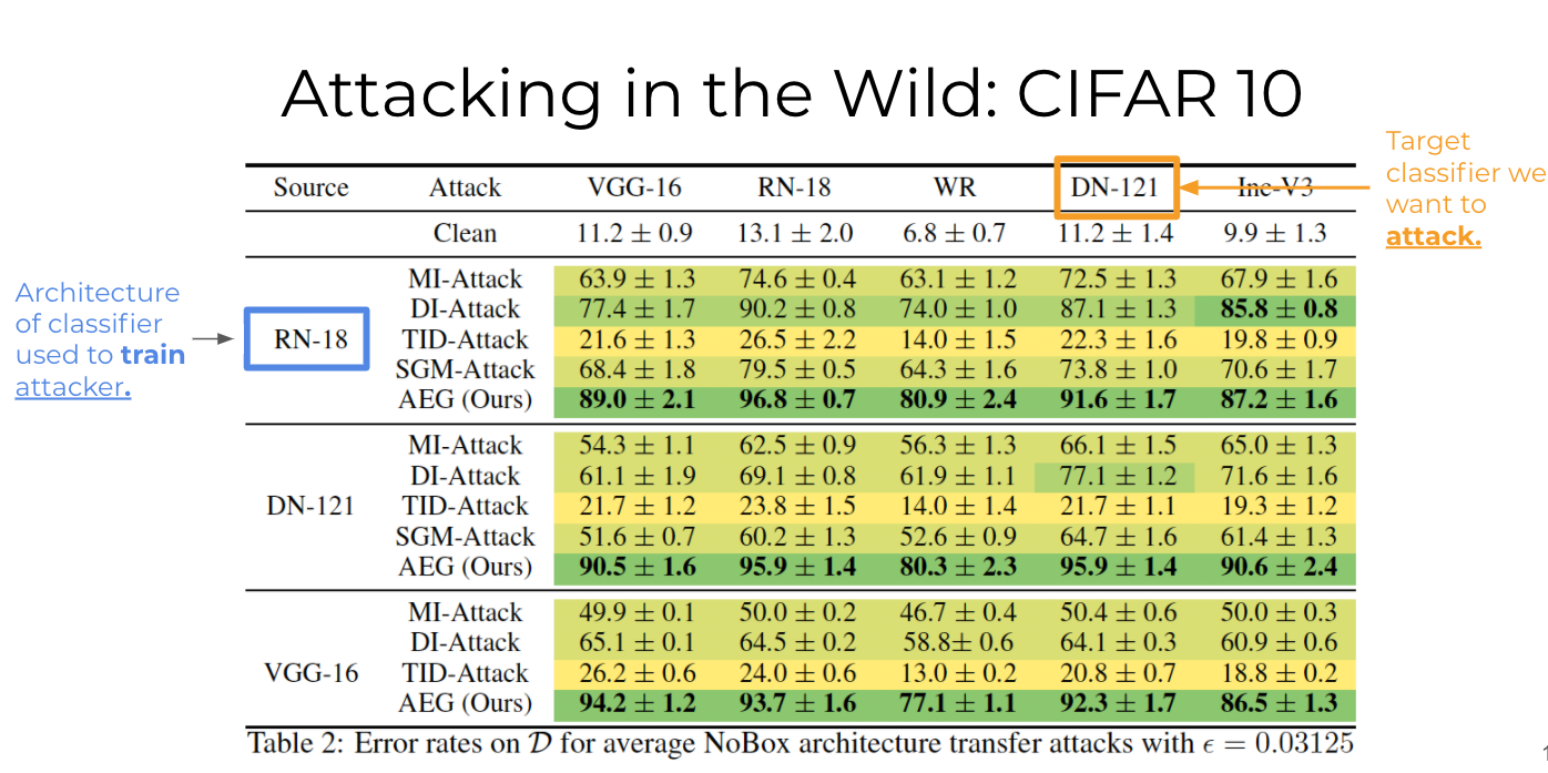
In this experiment we use the CIFAR-10 dataset and train \(10\) instances of VGG-16, ResNet-18 (RN-18), Wide ResNet (WR), DenseNet-121 (DN-121) and Inception-V3 architectures (Inc-V3). For baselines we considered previous BlackBox transfer methods that are popular in the literature. Without sounding too pompous, AEG completely obliterates the previous state of the art approaches and achieves impressively high attack success rate!

Conclusion

In this blogpost we’ve seen not only a new more realistic threat model (NoBox) but also a novel game theoretic framework for crafting attacks in this setting. While much of the theoretical and empirical details were glossed over in favor of lighter exposition they can be found in the full paper. Code for AEG is also available on the github repo. Looking into the future of adversarial attack research we hope that this new NoBox threat model provides a unique sandbox to experiment with newer adversarial attacks and also robustness strategies.